Benchmarks

This page tracks the canonical baseline numbers for OpenLithoHub's bundled ILT models, plus the differentiable forward models that drive them.

Headline baseline (synthetic-8)

Numbers are produced by

python scripts/generate_baselines.py --synthetic --limit 8 --output baselines/

against eight hand-rolled 64×64 layouts (square, h-line, line/space, T, L, cross, contacts, dense lines). The synthetic suite is dataset-free and runs in seconds, which is why it is the published reference. Real-dataset numbers can be regenerated locally with --data-root <path>.

Model	Samples	EPE mean (nm)	EPE max (nm)	PVB mean (nm)	MRC pass
dummy-identity	8	0.000	0.000	2.140	0%
rule-based-opc	8	0.530	1.414	2.487	0%
levelset-ilt (Gaussian PSF)	8	0.036	0.250	2.128	0%
neural-ilt (untrained U-Net)	8	15.074	24.637	2.497	100%

Things worth knowing about these numbers:

• dummy-identity copies the design straight through. Its EPE is zero by construction on a synthetic suite where design == target_mask. It exists as a smoke test of the metric pipeline, not as a real model.
• rule-based-opc applies analytic per-edge bias OPC. It is the cheapest non-trivial baseline and a fair starting point when comparing AI methods.
• levelset-ilt runs 200 iterations of gradient-descent ILT under the default Gaussian PSF forward model (sigma_px=2.0). The MRC failure count reflects the small synthetic patterns being narrower than the default min_width_nm=40; this is expected on a 64-pixel-wide canvas and not an indictment of the optimizer. Run with a real LithoBench layout or relaxed MRC thresholds for production-grade numbers.
• neural-ilt uses a randomly-initialized U-Net unless you load pretrained weights via the model hub. The EPE shown here is the honest "no-weights" baseline. It will improve substantially after training; we report it as-is rather than hide it.

Reproducing on real data

Once you have LithoBench cached locally:

python scripts/generate_baselines.py \
  --data-root /path/to/lithobench \
  --limit 16 \
  --pixel-nm 1.0 \
  --output baselines/lithobench/

The same results.json / results.md artifacts land under the chosen output directory. Submit them to the public leaderboard with openlithohub leaderboard submit --file <results.json>.

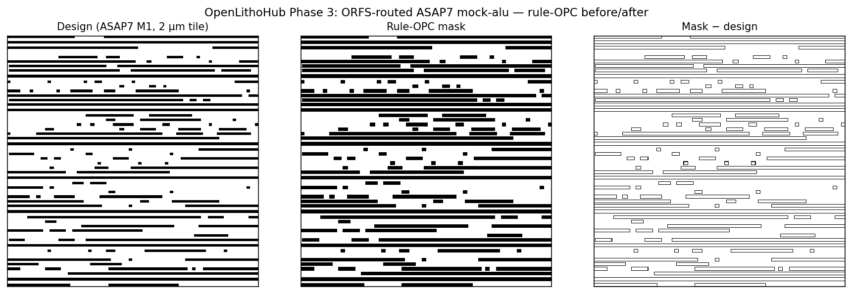
ORFS-routed ASAP7 — RISC-V mock-alu (issue #4 Phase 3)

OpenLithoHub also supports real ASAP7-routed RTL→GDSII outputs via the OrfsArtifactDataset adapter. The first end-to-end target is mock-alu from OpenROAD-flow-scripts: the smallest RISC-V-style ALU design that exercises a complete flow (yosys → OpenROAD → routed GDS) in ~25 minutes on a Linux runner.

The adapter rasterizes one design layer of the routed block, then cuts it into fixed-size tiles. The default 2 µm × 2 µm and 5 µm × 5 µm windows match the AI-OPC inference scales used in the literature.

To produce the GDS, trigger the build-asap7-mock-alu workflow (gh workflow run build-asap7-mock-alu.yml), download the artifact, and run:

.venv/bin/openlithohub eval run \
  --dataset orfs --node 7nm --accept-license \
  --data-root /path/to/6_final.gds \
  --tile-nm 2000 --pixel-nm 4.0 \
  --no-drc --no-mrc \
  --model dummy-identity

Window	Tiles total	PVB mean (nm)	PVB max (nm)
2 µm × 2 µm	729	15.073	29.600
5 µm × 5 µm	121	14.980	39.600

ORFS pinned at 74b5f96; metal1 layer 20/0; pixel_nm=4.0 (a 1 nm grid would be 16× more pixels and the PV-band convolution scales O(N²)). Linux-only locally — see scripts/build_riscv_alu.sh for the equivalent local commands.

Hotspot detection — ICCAD 2016 Problem C

The ICCAD'16 EUV hotspot benchmark is wired in via openlithohub.data.Iccad16Dataset (klayout-based OASIS rasterizer) and the point-matching metric compute_hotspot_detection. Together they support a separate baseline track from the mask-optimization numbers above — the data has no reference mask, so EPE / PVB / MRC do not apply.

Dataset

• 4 published test cases (testcase{1..4}.oas + test{1..4}.csv) mirrored at https://github.com/phdyang007/ICCAD16-N7M2EUV.
• Layer (1000, 0) is the design polygons; layer (10000, 0) is the hotspot-detection clip-site grid (16×16 nm windows, ~120 per case), exposed via LithoSample.metadata['clip_sites'].
• Hotspot annotations live in metadata['hotspots'] as (hotspot_id, category_id, x_nm, y_nm) rows. The contest's category-id-to-defect-kind mapping (EPE / Bridging / Necking) is not published, so the loader preserves the raw integer.
• LithoSample.mask is intentionally None for this dataset.

Metric

compute_hotspot_detection(predicted_points, ground_truth_points, match_radius_nm) does greedy point-matching: each predicted point counts as a TP iff an unmatched GT point lies within match_radius_nm. Returns {num_tp, num_fp, num_fn, recall, precision, f1}. Edge cases follow sklearn convention — empty-vs-empty is a vacuous perfect score; empty predictions against present GT give recall=0, precision=1.0.

Baselines

Sanity baselines (not ML predictors) are produced by:

python scripts/run_hotspot_baseline.py \
  --data-root data/iccad16 \
  --output out/hotspot \
  --match-radius-nm 100.0

Numbers below are from testcase1 (18 GT hotspots) at match_radius_nm=100 — the strict 1 nm radius is shown in the script's default output and gives all-zero TP for these strawman predictors.

Model	GT	Predicted	TP	FP	FN	Recall	Precision	F1
empty	18	0	0	0	18	0.000	1.000	0.000
grid-200nm	18	80	2	78	16	0.111	0.025	0.041
clip-centers	18	120	1	119	17	0.056	0.008	0.014

Things worth knowing:

• empty predicts nothing. It pins the recall floor (0.0) while scoring vacuous precision=1.0; useful as a "metric is alive" check.
• grid-200nm rasters predictions on a 200 nm lattice over the design bbox. Saturates the FP rate to expose the recall ceiling attainable by a brute-force "guess everywhere" predictor.
• clip-centers treats the auxiliary clip-site layer as a predictor. It performs near-zero — confirming our empirical finding that the clip-site grid is an inspection-window layer, not a hotspot mask. The 70+ nm separation between clip centers and CSV hotspots makes this baseline a useful regression check against anyone re-mistaking layer 10000 for ground truth.

A real ML predictor (CNN, ViT, etc.) plugs into the same script by adding a function to the PREDICTORS dict that consumes a LithoSample and returns an (N, 2) tensor of nm-coordinates.

GAN-OPC paired-mask dataset

openlithohub.data.GanOpcDataset exposes the ~4875 paired-PNG training set from Yang et al., GAN-OPC: Mask Optimization with Lithography-guided Generative Adversarial Nets (TCAD 2020). Source: https://github.com/phdyang007/GAN-OPC (multi-volume 7z archive, unpacks to ganopc-data/{artitgt,artimsk}/N.glp.png + N.glpOPC.png).

from openlithohub.data import GanOpcDataset

ds = GanOpcDataset("data/ganopc/extracted")  # parent of ganopc-data/
sample = ds[0]
sample.design  # (2048, 2048) torch.float32, {0., 1.}
sample.mask    # (2048, 2048) torch.float32, {0., 1.}

The pairs are (design_layout, OPC_mask) so this dataset is suitable for AI-OPC training and for evaluating mask-optimization models with the standard EPE / PVB / shot-count / MRC metric stack — though no canonical baseline numbers are published here yet.

Differentiable forward models

Two forward models ship in openlithohub._utils. Both are pure PyTorch and auto-differentiable, so they slot directly into ILT optimization loops, AI-OPC training, or any downstream gradient-based pipeline.

Gaussian PSF (default)

simulate_aerial_image(mask, sigma_px, dose=1.0) — a single Gaussian point spread function convolved with the mask. Fast, faithful enough for unit tests and small synthetic patterns, and used as the default in LevelSetILTModel.

Hopkins partial-coherent imaging (SOCS)

simulate_aerial_image_hopkins(mask, params) implements the Sum-of-Coherent- Systems decomposition of the Hopkins transmission cross coefficient. It captures partial coherence, off-axis illumination, and defocus, which the Gaussian model cannot.

Configurable via HopkinsParams:

Field	Default	Meaning
wavelength_nm	193.0	Exposure wavelength (193 nm = ArF, 13.5 nm = EUV)
na	1.35	Numerical aperture (image-side)
sigma	0.7	Partial-coherence factor; outer sigma for annular/dipole/quasar
sigma_inner	0.0	Inner sigma for off-axis illumination
pixel_size_nm	1.0	Physical mask pixel size
num_kernels	24	SOCS truncation order
illumination	"circular"	One of circular, annular, dipole, quasar
dipole_angle_deg	0.0	Pole-pair orientation for dipole/quasar
defocus_nm	0.0	Defocus offset (parabolic phase)

Switch LevelSetILTModel to Hopkins:

from openlithohub._utils import HopkinsParams
from openlithohub.models.levelset_ilt import LevelSetILTModel

model = LevelSetILTModel(
    iterations=200,
    forward_model="hopkins",
    hopkins_params=HopkinsParams(
        wavelength_nm=193.0,
        na=1.35,
        sigma=0.7,
        num_kernels=24,
        pixel_size_nm=2.0,
    ),
)
result = model.predict(design)  # standard PredictionResult

The kernels are computed once and cached per (params, grid_size, device), so iterative ILT loops pay the SVD cost a single time.